2.1. Step-by-step Example: Solving the XOR Problem
This tutorial introduces a basic and common usage of the primitiv by making and training a simple network for a small classification problem.
2.1.1. Introduction: Problem Formulation
Following lines are the formulation of the problem used in this tutorial:
where \(x_1, x_2 \in \mathbb{R}\). This is known as the XOR problem; \(f\) detects whether the signs of two arguments are same or not. We know that this problem is linearly non-separatable, i.e., the decision boundary of \(f\) can NOT be represented as a straight line on \(\mathbb{R}\): \(\alpha x_1 + \beta x_2 + \gamma = 0\), where \(\alpha, \beta, \gamma \in \mathbb{R}\).
For example, following code generates random data points \((x_1 + \epsilon_1, x_2 + \epsilon_2, f(x_1, x_2))\) according to this formulation with \(x_1, x_2 \sim \mathcal{N}(x; 0, \sigma_{\mathrm{data}})\) and \(\epsilon_1, \epsilon_2 \sim \mathcal{N}(\epsilon; 0, \sigma_{\mathrm{noise}})\):
#include <random>
#include <tuple>

class DataSource {
  std::mt19937 rng;
  std::normal_distribution<float> data_dist, noise_dist;

public:
  // Initializes the data provider with two SDs.
  DataSource(float data_sd, float noise_sd)
    : rng(std::random_device()())
    , data_dist(0, data_sd)
    , noise_dist(0, noise_sd) {}

  // Generates a data point
  std::tuple<float, float, float> operator()() {
    const float x1 = data_dist(rng);
    const float x2 = data_dist(rng);
    return std::make_tuple(
        x1 + noise_dist(rng),    // x1 + err
        x2 + noise_dist(rng),    // x2 + err
        x1 * x2 >= 0 ? 1 : -1);  // label
  }
};
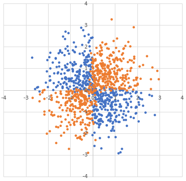
Following graph is an actual sample generated by above class with
data_sd is \(1\) and noise_sd is \(0.1\):
In this tutorial, we construct a 2-layers (input-hidden-output) perceptron to solve this problem. The whole model formulation is:
where \(y \in \mathbb{R}\) is an output value to be fit to \(f(x_1, x_2)\), \(\boldsymbol{x} := (x_1 \ x_2)^{\top} \in \mathbb{R}^2\) is an input vector, \(\boldsymbol{h} \in \mathbb{R}^N\) represents the \(N\)-dimentional hidden state of the network. There are also 4 free parameters: 2 matrices \(W_{hy} \in \mathbb{R}^{1 \times N}\) and \(W_{xh} \in \mathbb{R}^{N \times 2}\), and 2 bias (column) vectors \(b_y \in \mathbb{R}\) and \(\boldsymbol{b}_h \in \mathbb{R}^N\).
2.1.2. Include and Initialization
primitiv requires you to include primitiv/primitiv.h before using any
features in the source code.
All features in primitiv is enabled by including this header
(available features are depending on specified
options while building).
primitiv/primitiv.h basically may not affect the global namespace, and all
features in the library is declared in the primitiv namespace.
But for brevity, we will omit the primitiv namespace in this
tutorial using the using namespace directives.
Please pay attention to this point when you reuse these snippets.
#include <iostream>
#include <vector>
#include <primitiv/primitiv.h>

using namespace std;
using namespace primitiv;

int main() {

  // All code will be described here.

  return 0;
}
Before making our network, we need to create at least two objects: Device
and Graph.
Device objects specifies an actual computing backends (e.g., usual
CPUs, CUDA, etc.) and memory usages for these backends.
If you installed primitiv with no build options, you can initialize only
primitiv::devices::Naive device object.
Graph objects describe a temporary computation graph constructed by your
code and provides methods to manage their graphs.
devices::Naive dev;
Graph g;

// "Eigen" device can be enabled when -DPRIMITIV_USE_EIGEN=ON
//devices::Eigen dev;

// "CUDA" device can be enabled when -DPRIMITIV_USE_CUDA=ON
//devices::CUDA dev(gpu_id);
Note that Device and Graph is not a singleton; you can also create any
number of Device/Graph objects if necessary (even multiple devices share the
same backend).
After initializing a Device and a Graph, we set them as the default
device/graph used in the library.
Device::set_default(dev);
Graph::set_default(g);
For now, it is enough to know that these are just techniques to reduce coding efforts, and we don’t touch the details of ths function. For more details, please read the document about default objects.
2.1.3. Specifying Parameters and an Optimizer
Our network has 4 parameters described above:
\(W_{xh}\), \(\boldsymbol{b}_h\), \(W_{hy}\) and \(b_y\).
We first specify these parameters as Parameter objects:
constexpr unsigned N = 8;
Parameter pw_xh({N, 2}, initializers::XavierUniform());
Parameter pb_h({N}, initializers::Constant(0));
Parameter pw_hy({1, N}, initializers::XavierUniform());
Parameter pb_y({}, initializers::Constant(0));
Parameter objects basically take two arguments: shape and initializer.
Shapes specify actual volume (and number of free variables) in the parameter,
and initializer gives initial values of their variables.
Above code uses the
Xavier (Glorot) Initializer
for matrices, and the constant \(0\) for biases.
Next we initialize an Optimizer object and register all parameters to train
their values. We use simple SGD optimizer for now:
constexpr float learning_rate = 0.1;
optimizers::SGD opt(learning_rate);
opt.add(pw_xh, pb_h, pw_hy, pb_y);
2.1.4. Writing the Network
primitiv adopts the define-by-run style for writing neural networks.
Users can write their own networks as usual C++ functions.
Following code specifies the network described the above formulation using a
lambda functor which takes and returns Node objects:
// 2-layers feedforward neural network
// `x` should be with `Shape({2}, B)`
auto feedforward = [&](const Node &x) {
  namespace F = primitiv::functions;
  const Node w_xh = F::parameter<Node>(pw_xh);       // Shape({N, 2})
  const Node b_h = F::parameter<Node>(pb_h);         // Shape({N})
  const Node w_hy = F::parameter<Node>(pw_hy);       // Shape({1, N})
  const Node b_y = F::parameter<Node>(pb_y);         // Shape({})
  const Node h = F::tanh(F::matmul(w_xh, x) + b_h);  // Shape({N}, B)
  return F::tanh(F::matmul(w_hy, h) + b_y);          // Shape({}, B)
};
Node objects represent an virtual results of network calculations which are
returned by functions declared in the primitiv::functions namespace and can
be used as an argument of their functions. Each Node has a shape, which
represents the volume and the size of the minibatch of the Node.
primitiv encapsulates the treatment of minibatches according to the
minibatch broadcasting rule,
and users can concentrate on writing the network structure without considering
actual minibatch sizes.
We also describe a loss function about our network:
// Network for the squared loss function.
// `y` is that of returned from `feedforward()`
// `t` should be with `Shape({}, B)`
auto squared_loss = [](const Node &y, const Node &t) {
  namespace F = primitiv::functions;
  const Node diff = y - t;             // Shape({}, B)
  return F::batch::mean(diff * diff);  // Shape({})
};
Also, we write the network to generate input data from above DataSource
class:
constexpr float data_sd = 1.0;
constexpr float noise_sd = 0.1;
DataSource data_source(data_sd, noise_sd);

auto next_data = [&](unsigned minibatch_size) {
  std::vector<float> data;
  std::vector<float> labels;
  for (unsigned i = 0; i < minibatch_size; ++i) {
    float x1, x2, t;
    std::tie(x1, x2, t) = data_source();
    data.emplace_back(x1);
    data.emplace_back(x2);
    labels.emplace_back(t);
  }

  namespace F = primitiv::functions;
  return std::make_tuple(
      F::input<Node>(Shape({2}, minibatch_size), data),    // input data `x`
      F::input<Node>(Shape({}, minibatch_size), labels));  // label data `t`
};
primitiv::functions::input takes shape and actual data
(as a vector<float>) to make a new Node object.
The order of data should be the column-major order, and the minibatch is
treated as the last dimension w.r.t. the actual data.
For example, the Node with Shape({2, 2}, 3) has 12 values:
and the actual data should be ordered as:
2.1.5. Writing the Training Loop
Now we can perform actual training loop of our network:
for (unsigned epoch = 0; epoch < 100; ++epoch) {
  // Initializes the computation graph
  g.clear();

  // Obtains the next data
  Node x, t;
  std::tie(x, t) = next_data(1000);

  // Calculates the network
  const Node y = feedforward(x);

  // Calculates the loss
  const Node loss = squared_loss(y, t);
  std::cout << epoch << ": train loss=" << loss.to_float() << std::endl;

  // Performs backpropagation and updates parameters
  opt.reset_gradients();
  loss.backward();
  opt.update();
}
Above code uses Node.to_float(), which returns an actual single value stored
in the Node (this function can be used only when the Node stores just
one value).
You may get following results by running whole code described above (results may change randomly every time you launch the program):
0: loss=1.17221
1: loss=1.07423
2: loss=1.06282
3: loss=1.04641
4: loss=1.00851
5: loss=1.01904
6: loss=0.991312
7: loss=0.983432
8: loss=0.9697
9: loss=0.97692
...
2.1.6. Testing
Additionally, we launch a test process using a fixed data points in every 10 epochs:
- \((1, 1) \mapsto 1\)
- \((-1, 1) \mapsto -1\)
- \((-1, -1) \mapsto 1\)
- \((1, -1) \mapsto -1\)
for (unsigned epoch = 0; epoch < 100; ++epoch) {
  //
  // Training process written in the previous code block
  //

  if (epoch % 10 == 9) {
    namespace F = primitiv::functions;
    const Node test_x = F::input<Node>(Shape({2}, 4), {1, 1, -1, 1, -1, -1, 1, -1});
    const Node test_t = F::input<Node>(Shape({}, 4), {1, -1, 1, -1});
    const Node test_y = feedforward(test_x);
    const Node test_loss = squared_loss(test_y, test_t);
    std::cout << "test results:";
    for (float val : test_y.to_vector()) {
      std::cout << ' ' << val;
    }
    std::cout << "\ntest loss: " << test_loss.to_float() << std::endl;
  }
}
where Node.to_vector() returns all values stored in the Node.
Finally, you may get like below:
...
8: loss=0.933427
9: loss=0.927205
test results: 0.04619 -0.119208 0.0893511 -0.149148
test loss: 0.809695
10: loss=0.916669
11: loss=0.91744
...
18: loss=0.849496
19: loss=0.845048
test results: 0.156536 -0.229959 0.171106 -0.221599
test loss: 0.649342
20: loss=0.839679
21: loss=0.831217
...
We can see that the test results approaches correct values and the test loss becomes small by proceeding the training process.